Getting Started¶

Using BeamSection is straightforward, this section shows you how to calculate the beam properties step by step.

Graphical Interface¶

An overview of the Graphical User Interface (GUI) with notation is shown in the figure below.

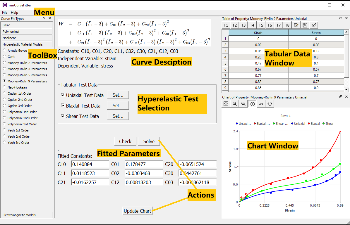
Menu¶

This section provides you basic actions in using CurveFitter. The actions include:

• Exit: Quits the program.
• Help: Runs your default web browser and visits official website welsim.com/curvefit.
• About: Displays About dialog and shows software and hardware information.

Toolbox¶

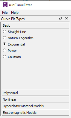
This section lists all available curves for you to choose from. The default curve is the straight line (first-order polynomial). The curves are grouped by the characteristics as follows.

Basic Curves¶

Straight line, Natural logarithm, Exponential, Power, Gaussian

Polynomial Curves¶

2^nd Order Polynomial, 3^rd Order Polynomial, 4^th Order Polynomial, 5^th Order Polynomial

Nonlinear Curves¶

Symmetrical Sigmoidal, Asymmetrical Sigmoidal, Rectangular Hyperbola, Basic Exponential, Half-Life Exponential, Proportional Rate Growth or Decrease

Hyperelastic Material Model Curves¶

Arruda-Boyce, Gent, Mooney-Rivlin 2, 3, 5, and 9 Parameters, Neo-Hookean, Ogden 1^st-3^rd Orders, Polynomial 1^st-3^rd Orders, Yeoh 1^st-3^rd Orders

Electromagnetic Model Curves¶

Electrical Steel, Power Ferrite

Curve Description¶

This section contains details about the selected curve, such as the function or energy functional, parameters to fit, variable descriptions.

For the hyperelastic model curves, additional Hyperelastic Test Data checkboxes shows in this seciton. It allows users to set/edit the test data at different deformations.

Fitted Parameters¶

This section outputs the fitted parameters for users. You also can edit the constants in the line edit widget and review the curves in the Chart window.

Actions¶

There are three actions provided for users to analyze or fit the test data.

• Check button: examines the input data in the tabular data window.
• Solve button: solves the curve fitting based on the input tabular data. The check process is implemented before the solution. If the curve fitting succeeded, the fitted constants will be set in the Fitted Parameters section, the curves will be plotted in the Chart window as well.
• Update Chart button: allows you to update the curves in the Chart window with the current constants.

Chart Windows¶

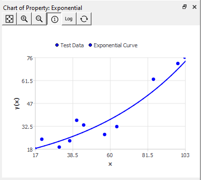
This section displays the test data dots and fitted curves in the same window, these dots and curves can be differentiated by legends and colors. Zoom in and out showing area are supported. You also can set the logarithmic axis for the curve display.

Workflow¶

This section demonstrates the procedures in applying curve fitting. The steps are followed:

1. Select the designated curve type from the toolbox.
   

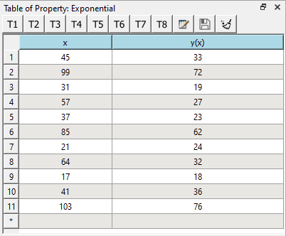
2. Edit table data or import data from an external file.
   

3. Review the test data in the Chart.
   

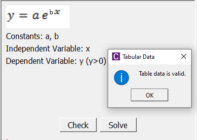
4. Check the input data (Optional). A pop-up message box indicates the status of the input data.
   

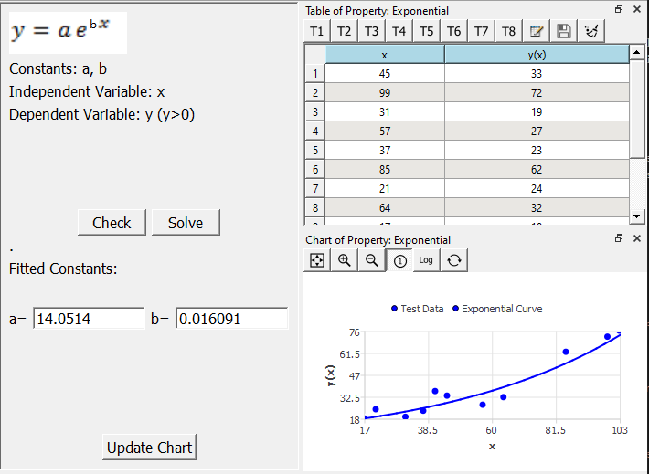
5. Solve the curves with the input tabular data. If it succeeded, the Constants line edits are filled with fitted parameters, and the Chart window displays the fitted curves along with the test data. These fitted parameters are the answers that we want.
   

6. Adjust parameters to evaluate the similar curves (Optional). You can change the parameters and hit the Update Chart button to see the new curves with modified parameters.