Core loss model¶

The core loss combines eddy current losses and hysteresis losses for a transient solution type. It is a post-processing calculation, based on already calculated transient magnetic field quantities. It is applicable for the evaluation of core losses in steel laminations (frequently used in applications such as electric machines, transformers) or in power ferrites.

Hysteresis loss is associated with loss density fields in 2D and 3D eddy current solutions only. Hysteresis loss is short for magnetic hysteresis loss and represents power loss in some magnetic materials (electric steels or ferrites) in alternating (sinusoidal) magnetic fields. This loss is due to a phenomenon called "magnetic viscosity" which causes the B and H fields to have a phase shift between them. In the B-H plane, for linear materials, the relationship between these two fields describes an ellipse. The hysteresis loss is proportional to the area of the ellipse.

Core loss models for an electromagnetic material¶

MatEditor provides two core loss models: electrical steel and power ferrite. The coefficients are given in the table below.

Type	Associated properties
Electrical Steel	Hystersis coefficient \(K_h\), Classcial eddy coefficient \(K_c\), Excess coefficient \(K_e\).
Power Ferrite	Steinmetz coefficients \(C_m\), \(X\), and \(Y\).

Note

In Transient Solver, X must be less than Y.

Calculating properties for core loss (B-P curve)¶

To be able to extract parameters from the loss characteristics (B-P Curve), you first set the Core Loss Model of the material to Electrical Steel or Power Ferrite as a material property in the Property View.

Additional parameters appear in the following table Core Loss Model (\(K_h\), \(K_c\), and \(K_e\) for electrical steel, and \(C_{m}\), \(X\), and \(Y\) for power ferrite). If the P-B test data is already presented in the current material, you can add curve fitting property from the RMB context menu. This allows the electrical steel coefficients \(K_h\), \(K_c\), and \(K_e\), or the power ferrite coefficients \(C_m\), \(X\), and \(Y\) to be derived from a manufacturer-provided core loss curve.

Node

The accuracy in inputting the data for B-P Curve for the electrical steel material has a significant effect on the correctness of the analyses to the electromagnetic devices. You should input the data for B-P Curve according to accurate data provided by material manufacturers. Typically core material suppliers provide the average loss over a cycle for a peak B, of sinusoidal nature. Therefore for BP curve input in WelSim, B (Tesla) should be peak and P should be average.

As the input data (value or unit) changes, the following parameters are not automatically updated unless you resolve the curve fitting:

\(K_h\) - Hysteresis Coefficient
\(K_c\) - Classical Eddy Coefficient
\(K_e\) - Excess Coefficient
\(C_m\) - Steinmetz Coefficient
\(X\) - Steinmetz Coefficient
\(Y\) - Steinmetz Coefficient

Calculate core loss coefficients from loss curves¶

This section introduces how to calculate core loss coefficients for electrical steel and power ferrite materials according to the given P-B test data.

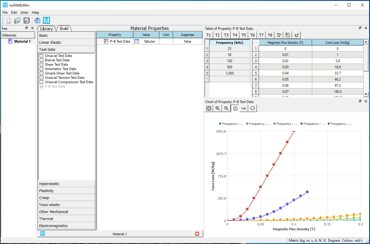
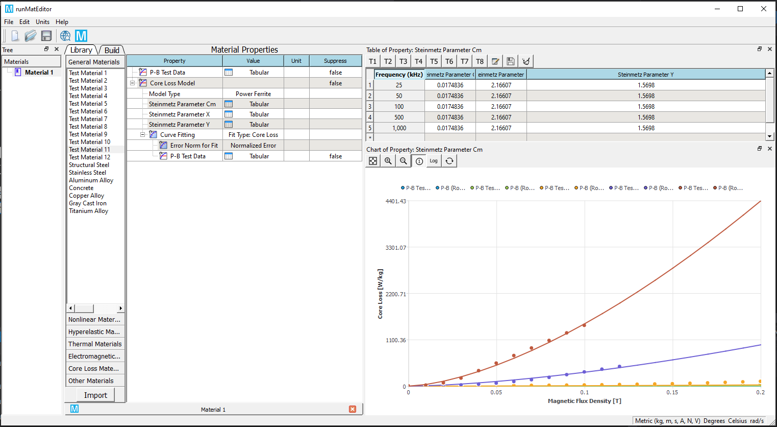
Add P-B Test Data material property, and edit the frequency-based data. You also can import the data from a plain text or Excel file. Check the data curves by clicking the row of frequency. Click the header of the frequency column displays all curves in the chart.
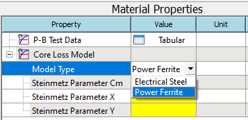
Add Core Loss Model material property, and set the Core Loss Model Type of the property to Electrical Steel or Power Ferrite.
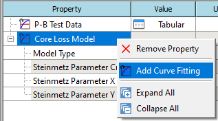
Add Curve Fitting sub-property from the RMB context menu.
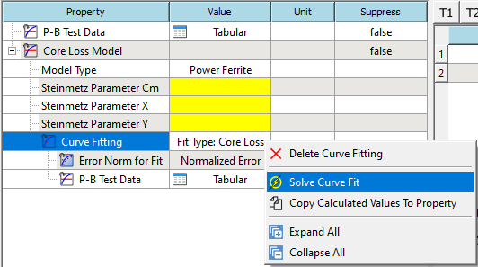
Solve the curve fit from the RMB context menu.
If the solve succeeds. The calculated parameters will be shown in the table.
Copy the solved values to the properties from RMB context menu. You also can review the calculated curves in the chart.
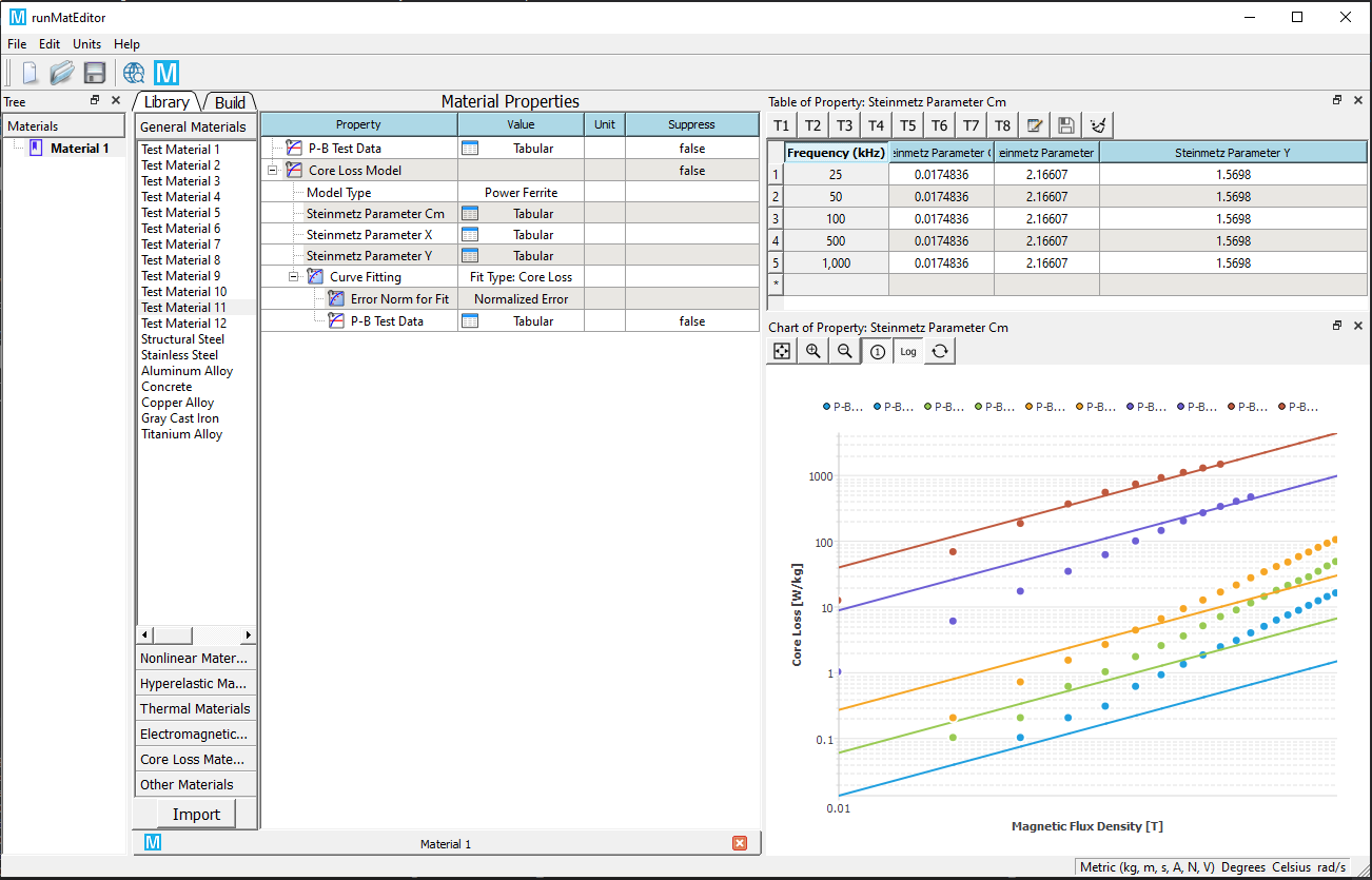
Display curves in the logarithmic axis (optional).

Computation of electrical steel core loss from loss curves¶

The iron-core loss without DC flux bias is expressed as the following:

\[ p_v=P_h+P_c+P_e=K_{f} f (B_m)^2 + K_c (fB_m)^2 + K_e(fB_m)^{1.5} = K_1B_m^2+K_2B_m^{1.5} \]

where

\(B_m\) is the amplitude of the AC flux component,
\(f\) is the frequency,
\(K_h\) is the hysteresis core loss coefficient,
\(K_c\) is the eddy-current core loss coefficient, and
\(K_e\) is the excess core loss coefficient,
\(K_1=K_ff+K_cf^2\),
\(K_2=K_ef^{1.5}\).

Minimize the quadratic form to obtain \(K_h\) , \(K_c\), and \(K_e\) directly.

\[ err(K_h,K_c,K_e)=\sum_{i=1}^m \sum_{j=1}^{n_i} \left[p_{ij}-\left(K_{h}f_{i}B_{mij}^2 +K_{c}\left(fB_{mij}\right)^{2}+ K_{e}\left(f_iB_{mij}\right)^{1.5} \right) \right]^2=min \]

where \(m\) is the number of loss curves, \(n_i\) is the number of points of the \(i\)-th loss curve, and \(p_{ij} = f(f_i , B_{mij})\) is two dimensional lookup table for loss curves.

Note

Since the manufacturer-provided loss curve is obtained under sinusoidal flux conditions at a given frequency, these coefficients can be derived in the frequency domain.

Computation of power ferrite core loss from loss curves¶

The principles of the computation algorithm are summarized as follows. The iron-core loss is expressed as the Steinmetz approximation

\[ p_v=C_m f^x B_m^y \]

where \(p_v\) is the average power density, \(f\) is the excitation frequency, and \(B_m\) is the peak flux density, is commonly used to characterize core loss data for sinusoidal excitation, but can also be applied to square-wave data.

To linearize the equation for curve fitting, we used base-10 logarithms. The equation above can be rewritten to

\[ log(p_v)=c + x\cdot log(f) + y \cdot(B_m) \]

where \(c=log(C_m)\).

Minimize the quadratic form to obtain \(C\), \(x\) and \(y\).

\[ err(C_m,x,y)=\sum_{i=1}^{m}\sum_{j=1}^{n_i}\left[log(p_{vij})-\left(c+xlog(f_i)+ylog(B_{mij}) \right) \right]^2=min \]

where \(m\) is the number of loss curves, \(n_i\) is the number of points of the \(i\)-th loss curve, and \(P_{vij} = f(f_i , B_{mij})\) is two dimensional lookup table for multi-frequency loss curves. Then \(C_m\) is calculated from the equation \(c=log(C_m)\).